Site Title

When you search on Amazon, YouTube, or Google, the system isn’t scanning every item one by one – it’s using ANN algorithms like HNSW to leap across billions of items in milliseconds. Modern search and LLM’s actively use hybrid search where semantic search augments keyword search. I have shared the intuition for semantic search in a previous post.

Semantic search deploys ANN (Approximate Nearest Neighbor) algorithms to navigate through billions of items to find the closest matching item. This post shares the general idea of ANN and presents the intuition for a popular ANN algorithm – HNSW (Highly Navigable Small World) used by vector search systems like FAISS, Pinecone, Weaviate to retrieve similar documents, images, or products in milliseconds,

Think of ANN as a super-smart post office for high-dimensional data, with a key caveat – it guarantees extremely fast routing of the mail but doesn’t guarantee the delivery to the exactly right address. It trades off perfect accuracy against speed. In other words, ANN is happy as long as the mail gets delivered to say, any home on the right street a.k.a. approximate nearest neighbor quickly. In most use cases where semantic search is deployed, this trade-off is acceptable – primarily because in most cases, there may not even be a perfect match.

• Meaning over Exact Words: Semantic search is all about matching the intended meaning or context of a user’s query, not the exact words. Real-world queries rarely correspond exactly to a single document or text fragment; instead, the user is looking for information that best answers his query – even if the words or phrasing are different.

• Perfect Match is Rare: In most practical scenarios, especially with large and diverse datasets, a perfect (word-for-word or context-for-context) match doesn’t exist. Users may phrase their queries differently from how content is indexed, or they may not know the precise terminology.

Part 1: What is HNSW? Think mail delivery system for Vectors
When mail delivery system sorts mail:
1. It goes from state → city → ZIP → street → house
2. Each step narrows down where the package should go.

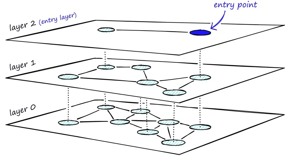
HNSW does exactly that with embeddings. Instead of brute-force comparing your query to all vectors, HNSW:

1. Builds a hierarchy of increasingly dense graphs
2. Starts the search from the highest level which is also the sparsest (like “state”), where it finds the closest match to incoming vector
3. Then the search lowers down to the next level from the closest match and repeats the process
4. The lowest layer has all the nodes or documents and search can finally find the approximate closest match to the incoming vector
5. Ends in dense layers (“house number”) to get a precise match

Part 2: How HNSW Inserts a New Vector

Let’s say you’re inserting product vector `V123`.

Step 1: Assign a Random Max Level

– V123 is randomly given a max level (say Level 3)
– It will be inserted into Levels 3, 2, 1, and 0

Step 2: Top down insertion

For each level from 3 → 0:

1. Use Greedy Search to find an entry point.
2. Perform `ef` Construction based search to explore candidates.
3. Select up to M nearest neighbors using a smart heuristic.
4. Connect bidirectionally (if possible).

Level 0 is the most important – it’s the dense, searchable layer. This is why HNSW powers semantic search in systems like FAISS and Pinecone – it’s how your query embedding finds the right chunk of meaning fast.

Part 3: Greedy vs `ef` Search – Why `ef` Matters

Say you’re at node P and evaluating neighbors A (8), B (5), and C (1), where the number in parentheses is the distance of point from the original vector – less means better match. Greedy search finds B is better than P and jumps to B – missing C, the true closest node.

With `ef = 3`, you:
– Evaluate A, B, and C
– Add all to candidate list
– Explore C later – and find the true best match

So `ef` controls how deeply and widely you explore:
– Greedy = fast, may miss best result
– `ef` search = slower, better accuracy

Part 4: What if a Node Already Has Max Neighbors?

When inserting a new node:
– It connects to M nearest neighbors
– Those neighbors may or may not link back

If a neighbor is already full:
– It evaluates if the new node is better than its current connections
– If so, it may drop a weaker link to accept the new one
– Otherwise, connection stays one-way only

This ensures:
– Graph remains navigable
– Degree of nodes stays bounded
– No constant link reshuffling

Final Thought

HNSW builds a navigable graph that scales to millions of vectors with:
– Fast approximate search
– Sparse yet connected layers
– Smart insertion and neighbor selection

So next time someone says “vector search,” remember the analogy of mail delivery system with a caveat of high speed with street level accuracy. Even if HNSW misses the absolute closest vector, retrieval pipelines typically fetch the top-k candidates, then rerank them with a more precise model. This way, speed and accuracy both stay high.